- The grammar of graphics
- Datasets and mapping
- Geometries
- Statistical transformation and plotting distribution
- Position adjustment and scales
- Coordinates and themes
- Facets and custom plots
View slides in new window
Presentation keyboard shortcuts
-
Use ← and → to navigate through the slides
-
Use F to toggle full screen
-
Use O to view an overview of all slides
-
Use ? to see a list of other shortcuts
Class demonstration
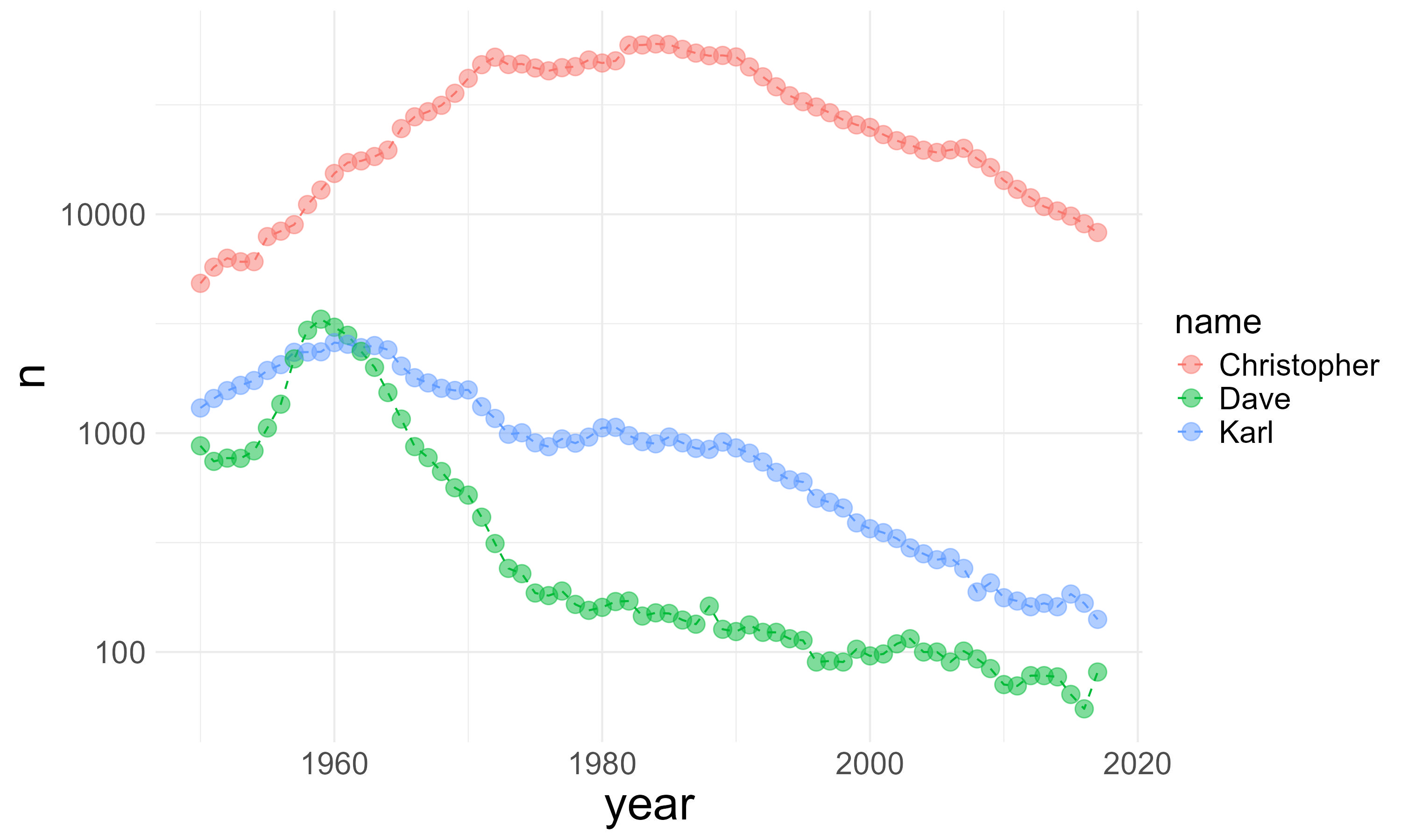
# libraries
library(tidyverse)
library(babynames)

## select names
friends <- babynames %>%
  filter(year >= 1950,
         name %in% c("Christopher", "Dave", "Karl"),
         sex == "M")

## plotting trends
ggplot(data = friends,
       mapping = aes(x = year, y = n, color = name)) +
  geom_line(linetype = "dashed") +
  geom_point(size = 4, alpha = 0.5) +
  scale_y_log10() +
  theme_minimal() +
  theme(axis.title = element_text(size = 24),
        axis.text = element_text(size = 16),
        legend.text = element_text(size = 16),
        legend.title = element_text(size = 18)
        )
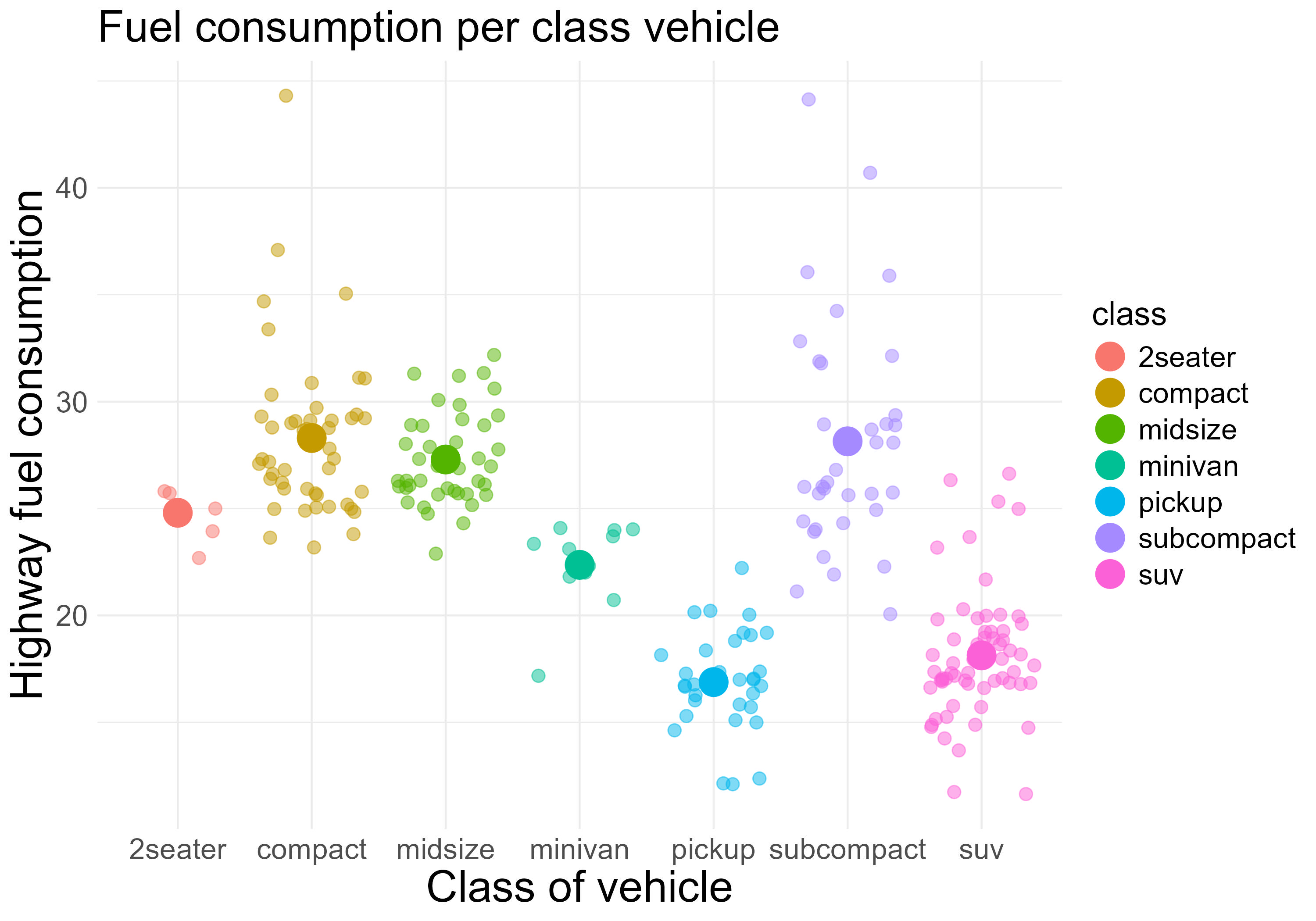
# libraries
library(tidyverse)

## calculating mean hwy per class
mean_hwy_data <- mpg %>%
  group_by(class) %>%
  summarise(mean_hwy = mean(hwy, na.rm = TRUE))

ggplot(data = mpg,
       mapping = aes(x = class, y = hwy, color = class)) +
  geom_point(position = "jitter", size = 3, alpha = 0.5) +
  geom_point(data = mean_hwy_data, aes(y = mean_hwy), size = 7) +
  labs(title = "Fuel consumption per class vehicle",
       x = "Class of vehicle",
       y = "Highway fuel consumption") +
  theme_minimal() +
  theme(plot.title = element_text(size = 24),
        axis.title = element_text(size = 24),
        axis.text = element_text(size = 16),
        legend.text = element_text(size = 16),
        legend.title = element_text(size = 18)
        )
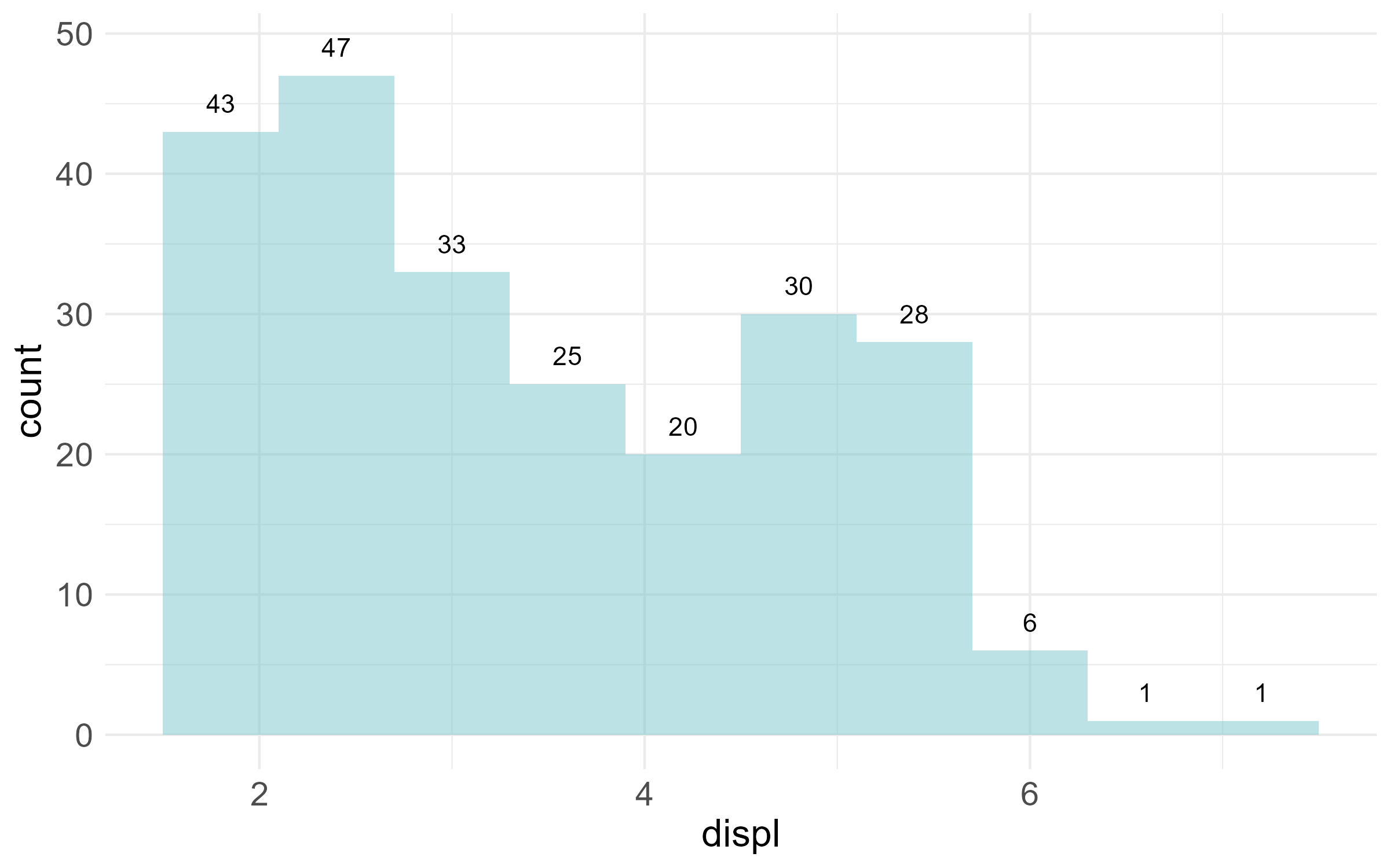
## libraries
library(tidyverse)

## histogram plot

ggplot(data = mpg,
       mapping = aes(x = displ)) +
  geom_histogram(bins = 10, fill = "cadetblue3", alpha = 0.5) +
  geom_text(aes(label = after_stat(count)),
            stat = "bin",
            bins = 10,
            nudge_y = 2) +
  theme_minimal() +
  theme(axis.text = element_text(size = 14),
        axis.title = element_text(size = 16),
        legend.text = element_text(size = 14),
        legend.title = element_text(size = 16)
        )